Sunday, March 27, 2016
Unit 4, Video 4 Summary
Loan-able funds graphs are easy to draw, interest rates go on the Y-Axis, Quantity goes on the X. There are two lines on the graph, supply of funds which slopes upward and demand for funds which slopes downward and the point they intersect at is the equilibrium. The supply of loan-able funds is dependent on savings. The more money people save, the more money banks have to loan. If the government runs at a deficit, then the demand for money will increase causing the interest rates to go up. The demand will shift to the right or increase. However, the supply of loan-able funds also increase because the supply of money is decreasing. Both can be shown on this graph but only one at a time as they mean roughly the same thing.

Unit 4, Video 6 Summary
It is important to keep all graphs labeled clearly. The three graphs that need to be tied together are the money market graphs, loan-able funds graph and the AD-AS graphs. Changes in the money market affect all of the other graphs. Most of the debt the government owes is to the people, not foreign countries. If the government demand for money increases in our money market graph to work out of a deficit, our interest rates also increase. On our loan-able funds graph, this either decreases our supply of loan-able fund or increases our demand for funds, both mean the same in this case. An increase in government demand causes an increase in AD on the AD-AS graphs which causes the GDP and price level to increase.
Unit 4, Video 5 Summary
The money creation process is how banks actually make money. Money is created by making loans. For example, if the reserve ratio is 20% and the loan amount is $500 is equal to a maximum creation of $2500 dollars in the money supply. This is figured out by multiplying the loan amount by the money multiplier, which is simply 1 over the Reserve ratio. The 2500 makes sense because it is all of the potential loans that could be made if one person withdraws the 500, places 400 into a bank and another withdraws, so on and so forth. This can only happen if there are no excess reserves in these banks. If the banks keep excess reserves, then the grand total of our $2500 is decreased.
Unit 4, Video 3 Summary
This video is over the Tools of Money Policy. There is expansionary which is easy money and contractionary which is tight money. To increase the money supply, reserve ratios(money held by banks) have to go down, along with the discount rate(rate a which banks can borrow money from FED). The opposite must happen to decrease the money supply(contraction). The most common thing banks do for either the creation or depletion of the money supply is buying or selling government bonds, respectively.
Unit 4; Video 2 Summary
Veal is tasty. This video is essentially practice over how to label a money market graph. on the Y-Axis, the price we pay to get money is labeled, AKA interest rate. On the X-Axis is labeled Quantity (of money). Demand will slope down(DM) due to the law of demand. The supply of money(SM) is vertical, because the supply of money is decided by the FED and does not fluctuate. A change in demand for money will shift the demand line either left or right. Changes in money supply will move the vertical line left or right.

Unit 4; Video 1 Summary
On the money market, there are three different types of money. First, there is commodity money which is what has been in use the longest and takes on the many forms such as crops or livestock. Second, there is representative money, which is money that represents something else, such as bills being representative of their equal amount in gold and silver. This kind of money is severely unstable as the worth fluctuates. Thirdly, there is fiat money. This money is not backed by anything except the word of the government, and must be accepted for transaction. Money has three functions as mediums of exchange, store of value and unit of account showing that price has worth(more expensive gives impression of higher quality).
Friday, March 4, 2016
Unit 3; Day 6- Fiscal Policy
Fiscal Policy-Changes in expenditures or tax revenues of the federal government
2 tools of fiscal policy- taxes gov can increase decrease; spending gov can increase decrease
More info. on FP
Fiscal Policy Video
Balanced budget
Revenues= expenditures
Budget deficit
Revenues< expenditures
Budget surplus
Revenues > expenditures
Govt debt= sum of all deficits - sum of all surplus
Government must borrow when in deficit
From individuals, corporations, financial institutions, foreign entities
Discretionary fiscal policy (action)
Expansionary= deficit
Contractionary= surplus
Non-discretionary policy (no action)
Discretionary- increase or decrease gov spending and/or taxes in order to return the economy to full employment. Discretionary policy involves policy makers doing fiscal policy in response to an economic problem
Automatic- unemployment compensation and marginal tax rates are examples of automatic policy that help mitigate the effects of recession and inflation. Automatic fiscal takes place without policy makers having to respond to current economic problems
Expansionary - “easy” combat recession, increase gov spending, lower taxes
Contractionary- “tight” combat Inflation on, lower gov spending, increase taxes
Automatic or built in stabilizers-
Anything that increases gov budget deficit during a recession and increases it's budget surplus during inflation without requiring explicit action by policymakers
Unemployment comp.
Welfare and social security
Medicare medicaid
VA benefits
Progressive tax system
Average tax rate(tax revenue/gdp) rises with gdp
Proportional tax system
Average tax rate remain constant as gdp changes
Regressive tax system
Average tax rate falls with gdp
2 tools of fiscal policy- taxes gov can increase decrease; spending gov can increase decrease
More info. on FP
Fiscal Policy Video
Balanced budget
Revenues= expenditures
Budget deficit
Revenues< expenditures
Budget surplus
Revenues > expenditures
Govt debt= sum of all deficits - sum of all surplus
Government must borrow when in deficit
From individuals, corporations, financial institutions, foreign entities
Discretionary fiscal policy (action)
Expansionary= deficit
Contractionary= surplus
Non-discretionary policy (no action)
Discretionary- increase or decrease gov spending and/or taxes in order to return the economy to full employment. Discretionary policy involves policy makers doing fiscal policy in response to an economic problem
Automatic- unemployment compensation and marginal tax rates are examples of automatic policy that help mitigate the effects of recession and inflation. Automatic fiscal takes place without policy makers having to respond to current economic problems
Expansionary - “easy” combat recession, increase gov spending, lower taxes
Contractionary- “tight” combat Inflation on, lower gov spending, increase taxes
Automatic or built in stabilizers-
Anything that increases gov budget deficit during a recession and increases it's budget surplus during inflation without requiring explicit action by policymakers
Unemployment comp.
Welfare and social security
Medicare medicaid
VA benefits
Progressive tax system
Average tax rate(tax revenue/gdp) rises with gdp
Proportional tax system
Average tax rate remain constant as gdp changes
Regressive tax system
Average tax rate falls with gdp
Unit 3; Day 5- Consumption Spending and Saving
Disposable Income - Income after taxes or net income
DI= Gross income- Taxes
2 Choices
Consume(spend on goods and services)-
Household spending
The ability to consume constrained by- amount of DI, Propensity to save
Do households consume if DI=0? Autonomous Consumption
Save(Not spend on goods and services)-
Household NOT spending
Ability to save is constrained by- amount of DO, Propensity to consume
Do households save if DI=0? No
APC & APS
Consumption/DI= APC
APC + APS=1
1-APC= APS
1-APS=APC
APC>1~ Dissaving
Negative APS~ dissaving
Marginal Propensity to Consume (MPC)- Fraction of any change in DI that is consumed
=Δconsumption/ Δ DI
Marginal Propensity to Save (MPS)- Fraction of Change in DI that is saved
=Δ savings/ Δ DI
MPC+MPS=1
1-MPS= MPC
1-MPC=MPS (People can only consume or save Disposable income)
Tax Multiplier= -MPC/MPS
Govt Spending Multiplier= 1/MPS
The Spending multiplier Effect- An initial change in spending( C,Ig, G, Xn) causes a larger change in Aggregate spending(AS), or Aggregate Demand(AD)
Multiplier= Δ AD/ Δ spending
Calculating the Spending Multiplier- can be calc. from the MPC or MPS
Multiplier= 1/(1-MPC) or 1/MPS
Positive when there is increase in spending, negative when decrease
Calculating the Tax Multiplier- When Govt. taxes, multiplier works reverse. Why? Money is now leaving circular flow.
Tax multiplier(it is negative)= -MPC/(1-MPC) or -MPC/MPS
If there is a tax cut, multiplier is negative; more money in circular flow
DI= Gross income- Taxes
2 Choices
Consume(spend on goods and services)-
Household spending
The ability to consume constrained by- amount of DI, Propensity to save
Do households consume if DI=0? Autonomous Consumption
Save(Not spend on goods and services)-
Household NOT spending
Ability to save is constrained by- amount of DO, Propensity to consume
Do households save if DI=0? No
APC & APS
Consumption/DI= APC
APC + APS=1
1-APC= APS
1-APS=APC
APC>1~ Dissaving
Negative APS~ dissaving
Marginal Propensity to Consume (MPC)- Fraction of any change in DI that is consumed
=Δconsumption/ Δ DI
Marginal Propensity to Save (MPS)- Fraction of Change in DI that is saved
=Δ savings/ Δ DI
MPC+MPS=1
1-MPS= MPC
1-MPC=MPS (People can only consume or save Disposable income)
Tax Multiplier= -MPC/MPS
Govt Spending Multiplier= 1/MPS
The Spending multiplier Effect- An initial change in spending( C,Ig, G, Xn) causes a larger change in Aggregate spending(AS), or Aggregate Demand(AD)
Multiplier= Δ AD/ Δ spending
Calculating the Spending Multiplier- can be calc. from the MPC or MPS
Multiplier= 1/(1-MPC) or 1/MPS
Positive when there is increase in spending, negative when decrease
Calculating the Tax Multiplier- When Govt. taxes, multiplier works reverse. Why? Money is now leaving circular flow.
Tax multiplier(it is negative)= -MPC/(1-MPC) or -MPC/MPS
If there is a tax cut, multiplier is negative; more money in circular flow
Unit 3; Day 4- Classical Vs. Keynesian
Video on Classical vs. Keynesian
Classical School-
Modern Followers- Adam Smith, Alfred Marshall, JB Say, David Ricardo
Say's Law- Supply always creates its own demand.
Production=income=spending; under spending is unlikely
Whatever output produced will be demanded.
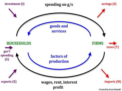
Savings= Investment income, Saving(leakage)= Investment(Injection)
Competition good
Government-
Invisible Hand- Govt/econ. can regulate self
Monetary rule
maintains steady money supply
Laissez-Faire
Economy-
Economy self regulating
In long run, economy will balance at full employment.
Economy is always close to or full employment
Unemployment rarely exists due to wage, price flexibility
Prices, wages are flexible downward
Support trickle-down effect (rich first, everyone else second)
Supply curve- Vertical
AS determines output, employment
AD determines price level, reasonably stable if money supply is stable.
MV=P*Q
SRAS is short, Emphasis today in Microeconomics
Keynesian School-
Competition flawed
AD is key, not AS
Leaks and savings cause recession
Government
Fiscal Policy- Tax and spend
Believe in active government
Economy is no self-regulating
Economy
C+Ig+G+Xn=GDP
AD determines output and employment
Ratchet effects+ Sticky wages block Say’s Law.
Prices and wages inflexible downward
Unemployment usually exists, caused by external and internal
Inflation is caused by too much demand
SRAS is long, Emphasis today in macroecnomics. In long run, we are dead.
Classical School-
Modern Followers- Adam Smith, Alfred Marshall, JB Say, David Ricardo
Say's Law- Supply always creates its own demand.
Production=income=spending; under spending is unlikely
Whatever output produced will be demanded.
Savings= Investment income, Saving(leakage)= Investment(Injection)
Competition good
Government-
Invisible Hand- Govt/econ. can regulate self
Monetary rule
maintains steady money supply
Laissez-Faire
Economy-
Economy self regulating
In long run, economy will balance at full employment.
Economy is always close to or full employment
Unemployment rarely exists due to wage, price flexibility
Prices, wages are flexible downward
Support trickle-down effect (rich first, everyone else second)
Supply curve- Vertical
AS determines output, employment
AD determines price level, reasonably stable if money supply is stable.
MV=P*Q
SRAS is short, Emphasis today in Microeconomics
Keynesian School-
Competition flawed
AD is key, not AS
Leaks and savings cause recession
Government
Fiscal Policy- Tax and spend
Believe in active government
Economy is no self-regulating
Economy
C+Ig+G+Xn=GDP
AD determines output and employment
Ratchet effects+ Sticky wages block Say’s Law.
Prices and wages inflexible downward
Unemployment usually exists, caused by external and internal
Inflation is caused by too much demand
SRAS is long, Emphasis today in macroecnomics. In long run, we are dead.
Unit 3; Day 3- Investment
Investment- money spent or expenditures on:
New plants(factory)
Capital Equipment(Machinery)
Technology(hardware/software)
New Homes
Inventories(goods sold by producers)
Expected Rates of Return-
How does business make investment decisions? Cost/ Benefit Analysis
How does a business determine benefit? Expected rate of return
How does business count cost? Interest Costs
How does business determine the amount of investment they undertake? Compare expected rate of return to interest cost.
If expected return> interest cost, then invest
If expected return< interest cost, do not invest
Real(r%) vs. Nominal(i%)
What’s the difference?
Nominal is the observable rate of interest.
Real subtracts out inflation(pi%) and is only known ex post facto.
How do you compute the real interest rate(r%)?
r%-i%-pi%
What then, determines the cost of an investment decision?
The real interest rate(r%)
~
Investment demand curve- Downward sloping.
Why? When interest rates are high, fewer investments are profitable; when interest rates are low, more investments are profitable.
Shifts in Investment Demand
Cost of production
Lower costs shift ID>
Higher costs shift ID<
Business taxes
Lower taxes ID>
Higher taxes ID<
Technological Change
New tech ID>
Lack of tech ID<
Stock of Capital
Low capital ID>
High Capital ID<
Expectations
Positive expect. ID>
Negative Expect ID<
New plants(factory)
Capital Equipment(Machinery)
Technology(hardware/software)
New Homes
Inventories(goods sold by producers)
Expected Rates of Return-
How does business make investment decisions? Cost/ Benefit Analysis
How does a business determine benefit? Expected rate of return
How does business count cost? Interest Costs
How does business determine the amount of investment they undertake? Compare expected rate of return to interest cost.
If expected return> interest cost, then invest
If expected return< interest cost, do not invest
Real(r%) vs. Nominal(i%)
What’s the difference?
Nominal is the observable rate of interest.
Real subtracts out inflation(pi%) and is only known ex post facto.
How do you compute the real interest rate(r%)?
r%-i%-pi%
What then, determines the cost of an investment decision?
The real interest rate(r%)
~
Investment demand curve- Downward sloping.
Why? When interest rates are high, fewer investments are profitable; when interest rates are low, more investments are profitable.
Shifts in Investment Demand
Cost of production
Lower costs shift ID>
Higher costs shift ID<
Business taxes
Lower taxes ID>
Higher taxes ID<
Technological Change
New tech ID>
Lack of tech ID<
Stock of Capital
Low capital ID>
High Capital ID<
Expectations
Positive expect. ID>
Negative Expect ID<
Unit 3; Day 2- Aggregate Supply
Aggregate Supply- Level of Real GDP that firms produce at price level

Long-Run- Period of time where input prices are completely flexible; adjust to changes in price level. Level of real gdp supplied is independent price level.
Short-Run- Period of time where input prices are sticky; do not adjust to changes in price level. Level of real gdp supplied directly related to price level
Long Run Aggregate Supply(LRAS)- marks level of full employment in economy (analogous to PPC)
Because input prices are completely flexible, changes in price level do not change firms’ real profits and therefore do not change firms’ level of output. This means that LRAS is vertical at economy’s lvl of employment.
Short Run Aggregate Supply(SRAS)- increase in SRAS= shift to right. ->; Decrease in SRAS is seen as shift to the left. SRAS<-
Key unit to understanding shifts is per unit cost of produc. = total input cost (input*price per unit)/ total output

Things that affect SRAS
Input Prices-
Domestic resource prices-
Wages(75% business costs)
cost ofcapital
raw materials(commodity prices)
Foreign resource prices-
Strong$= lower foreign resources prices
Weak$= Higher foreign resource prices
Market power
Increases in resource prices= SRAS<-
Decrease in resource prices= SRAS->
Productivity= Total output/ total input
More productivity= lower unit produc. cost= SRAS>
Lower productivity= higher unit produc. cost= SRAS<
Taxes and Subsidies
Taxes($ to govt) on business increase per unit produc. cost= SRAS<
Subsidies($ from gov) to business reduce produc. cost= SRAS>
Government regulation
Govt regulation creates cost compliance= SRAS<
Deregulation reduces compliance costs= SRAS>
~
Full Employment
Equilibrium exists where AD intersects SRAS and LRAS at same point.
Recessionary Gap
Exists when equilibrium occurs below full employment output.
Inflationary Gap
Exists when equilibrium occurs beyond full employment output
~
Nominal wages- Amount of money received by a worker per unit of Time
Real Wage- amount of goods and services a worker can purchase with their nominal wages. In essence, real wage is the purchasing power of nominal
Sticky wage- Amount set based on initial price level and does not vary due to labor contracts or other restrictions.
Long-Run- Period of time where input prices are completely flexible; adjust to changes in price level. Level of real gdp supplied is independent price level.
Short-Run- Period of time where input prices are sticky; do not adjust to changes in price level. Level of real gdp supplied directly related to price level
Long Run Aggregate Supply(LRAS)- marks level of full employment in economy (analogous to PPC)
Because input prices are completely flexible, changes in price level do not change firms’ real profits and therefore do not change firms’ level of output. This means that LRAS is vertical at economy’s lvl of employment.
Short Run Aggregate Supply(SRAS)- increase in SRAS= shift to right. ->; Decrease in SRAS is seen as shift to the left. SRAS<-
Key unit to understanding shifts is per unit cost of produc. = total input cost (input*price per unit)/ total output
Things that affect SRAS
Input Prices-
Domestic resource prices-
Wages(75% business costs)
cost ofcapital
raw materials(commodity prices)
Foreign resource prices-
Strong$= lower foreign resources prices
Weak$= Higher foreign resource prices
Market power
Increases in resource prices= SRAS<-
Decrease in resource prices= SRAS->
Productivity= Total output/ total input
More productivity= lower unit produc. cost= SRAS>
Lower productivity= higher unit produc. cost= SRAS<
Taxes and Subsidies
Taxes($ to govt) on business increase per unit produc. cost= SRAS<
Subsidies($ from gov) to business reduce produc. cost= SRAS>
Government regulation
Govt regulation creates cost compliance= SRAS<
Deregulation reduces compliance costs= SRAS>
~
Full Employment
Equilibrium exists where AD intersects SRAS and LRAS at same point.
Recessionary Gap
Exists when equilibrium occurs below full employment output.
Inflationary Gap
Exists when equilibrium occurs beyond full employment output
~
Nominal wages- Amount of money received by a worker per unit of Time
Real Wage- amount of goods and services a worker can purchase with their nominal wages. In essence, real wage is the purchasing power of nominal
Sticky wage- Amount set based on initial price level and does not vary due to labor contracts or other restrictions.
Unit 3; Day 1- Aggregate Demand
Aggregate Demand Curve =C+I+G+Xn
Price lvl = Y, Real GDP= X; There is an inverse relationship between X and Y.

AD is the demand by consumers, businesses, government, and foreign countries.
What definitely doesn’t shift the curve?
Changes in price level cause a move along the curve.
Why is AD downward sloping?
1. Real balance effect-
Higher price levels reduce the purchasing power of money
This decreases the quantity of expenditures
Lower price levels increase purchasing power and increase and expenditures
2. Interest Rate effect-
When the price level increases, lenders need to charge higher interest rates to get a REAL return on their loans.
Higher interest rates discourage consumer spending and business investment.
3. Foreign Trade Effect
When US price level rises, foreign buyers purchase fewer US goods and Americans buy more foreign goods.
Exports fall and imports rise, causing real GDP to fall. (Xn decreases)
Shifters of aggregate Demand: GDP= C+I+G+Xn
There are two parts to a shift in AD
A change in C, I, G, and/or Xn
A multiplier effect that produces a greater change than original change in 4 components
Increase in AD= AD->
Decrease in AD= <-AD
Determinants of AD-
Consumption
Household spending is affected by:
Consumer wealth. More wealth= more spending(AD ->), less wealth= less spending
Consumer Expectations. Positive expectations= more spending, Neg.= less spending
Household indebtedness. Less debt= more spending, more debt= less spending
Taxes. Less taxes, more spending, more taxes, less spending
Gross Private Domestic Investment
Investment spending is sensitive to:
Real Interest rate. Lower rate= more investment(AD->); higher Real interest rate= Less investment
Expected returns. Higher expected returns= More investment, Lower Expected returns= less investment
Influenced by-
Expectations of future profitability,
Tech
Degree of excess capacity(Existing stock of capital)
Business taxes
Net Exports
Sensitive to
Exchange rates. Strong $= more imports. less exports. (AD<). Weak$= Fewer imports, more exports (AD>)
Relative income. Strong foreign economies= more exports (AD>). Weak foreign economies= less imports (AD<)
Price lvl = Y, Real GDP= X; There is an inverse relationship between X and Y.
AD is the demand by consumers, businesses, government, and foreign countries.
What definitely doesn’t shift the curve?
Changes in price level cause a move along the curve.
Why is AD downward sloping?
1. Real balance effect-
Higher price levels reduce the purchasing power of money
This decreases the quantity of expenditures
Lower price levels increase purchasing power and increase and expenditures
2. Interest Rate effect-
When the price level increases, lenders need to charge higher interest rates to get a REAL return on their loans.
Higher interest rates discourage consumer spending and business investment.
3. Foreign Trade Effect
When US price level rises, foreign buyers purchase fewer US goods and Americans buy more foreign goods.
Exports fall and imports rise, causing real GDP to fall. (Xn decreases)
Shifters of aggregate Demand: GDP= C+I+G+Xn
There are two parts to a shift in AD
A change in C, I, G, and/or Xn
A multiplier effect that produces a greater change than original change in 4 components
Increase in AD= AD->
Decrease in AD= <-AD
Determinants of AD-
Consumption
Household spending is affected by:
Consumer wealth. More wealth= more spending(AD ->), less wealth= less spending
Consumer Expectations. Positive expectations= more spending, Neg.= less spending
Household indebtedness. Less debt= more spending, more debt= less spending
Taxes. Less taxes, more spending, more taxes, less spending
Gross Private Domestic Investment
Investment spending is sensitive to:
Real Interest rate. Lower rate= more investment(AD->); higher Real interest rate= Less investment
Expected returns. Higher expected returns= More investment, Lower Expected returns= less investment
Influenced by-
Expectations of future profitability,
Tech
Degree of excess capacity(Existing stock of capital)
Business taxes
Net Exports
Sensitive to
Exchange rates. Strong $= more imports. less exports. (AD<). Weak$= Fewer imports, more exports (AD>)
Relative income. Strong foreign economies= more exports (AD>). Weak foreign economies= less imports (AD<)
Subscribe to:
Posts (Atom)